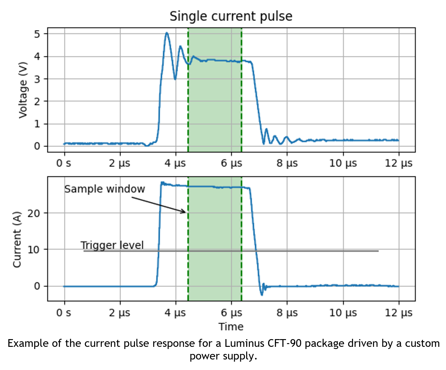
Electrical - How do I simulate an LED pulse in Spice? – Luminus Devices

First, we start with an example of a real pulse measurement of a Luminus CFT-90 LED package to define a good model response.

This type of measurement has a strong interaction with the power supply design and often the waveforms of real measurements reflect the frequency response characteristics of the power supply. This particular power supply was custom built to deliver relatively clean current pulses up to 50 A and measure the voltage response with minimal junction heating.

The rise and fall times for this type of LED have been determined using other measurements as around
25 ns and we can see that the slopes of the input current pulse closely match those of the output voltage waveform. This implies that the LED frequency response is much faster than this particular power supply. The ringing in the waveforms are due to small inductances which have been minimized in this power supply and header design.

The objective of this article is to demonstrate how to model pulses with Spice models. We find that pulsing with a voltage source is straightforward but pulsing with a current source requires adjustment of the model parameters. There are a number of issues related to hidden default settings and digitization that need to be addressed.

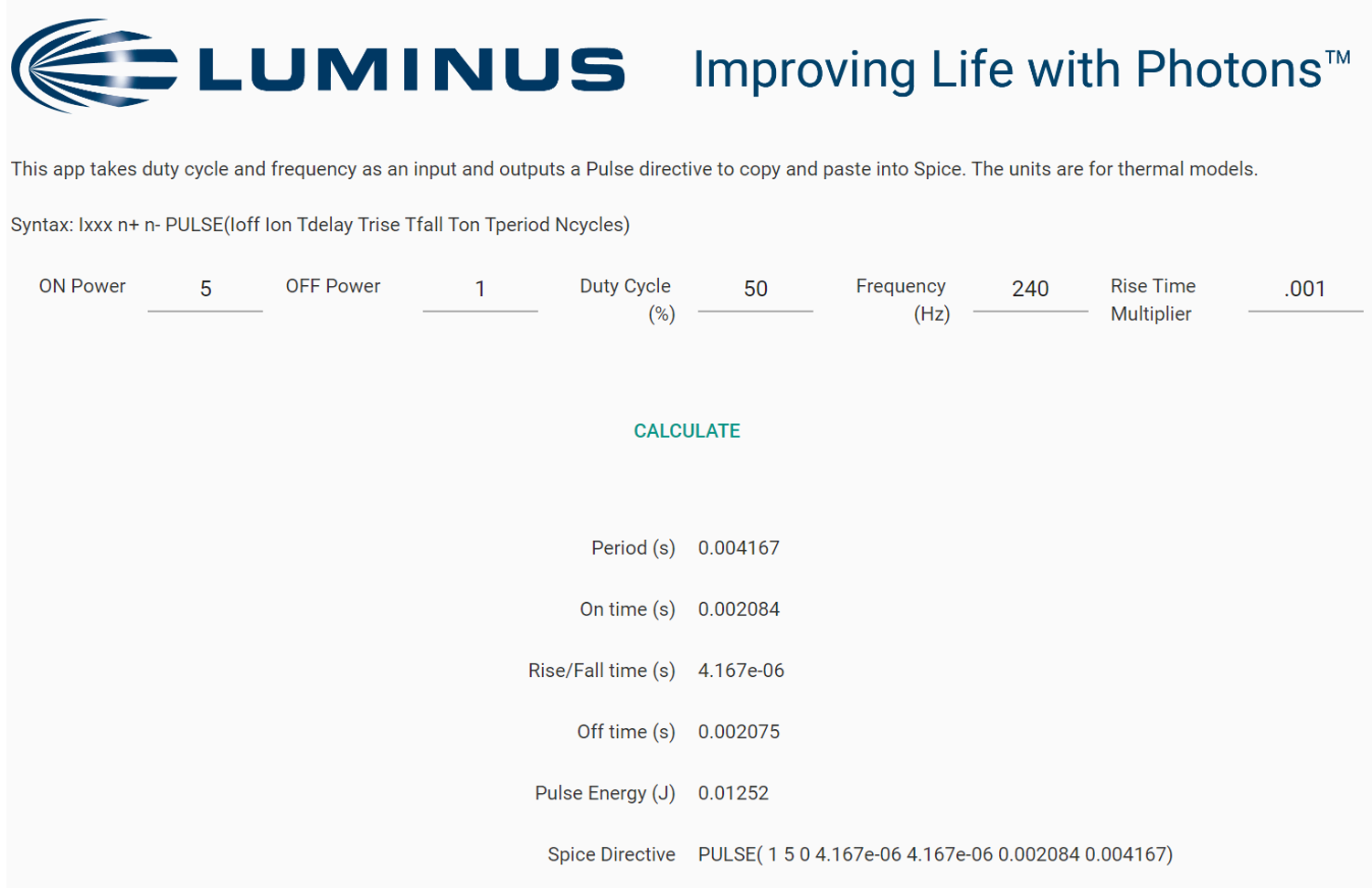
Spice uses a PULSE command that has a syntax of PULSE(Ioff, Ion, Tdelay, Trise, Tfall, Ton, Tperiod, Ncycles). Most LED people think about duty cycle and frequency, and as a convenience the link below presents an App that calculates and displays the equivalent Spice command for duty cycle – frequency – amplitude parameters that you can copy-paste into your model. “Spice - Duty Cycle and Frequency to Spice Command”.

The figure below shows the IV curves and pulse response for a typical blue LED rated for 120 mA maximum current. We expect the output waveforms to closely follow the inputs for this relatively slow pulse.

The pulse response for the voltage source is well behaved but the pulse response of the current source is not. The reason this happens is a combination of digitization artifacts and hidden defaults in the Spice calculation code that are included to optimize convergence speed and prevent singularities.

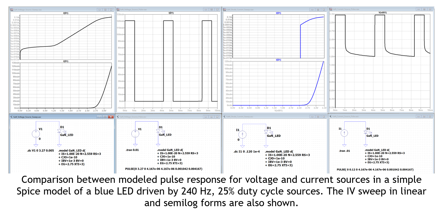
The digitization effect can be observed in the semilog IV plots. The voltage sweep starts at zero and has a 5-mV step size. The first non-zero datapoint is calculated for 5 mV and has a calculated current near 1e-15 A. This produces a smooth curve that starts at zero.

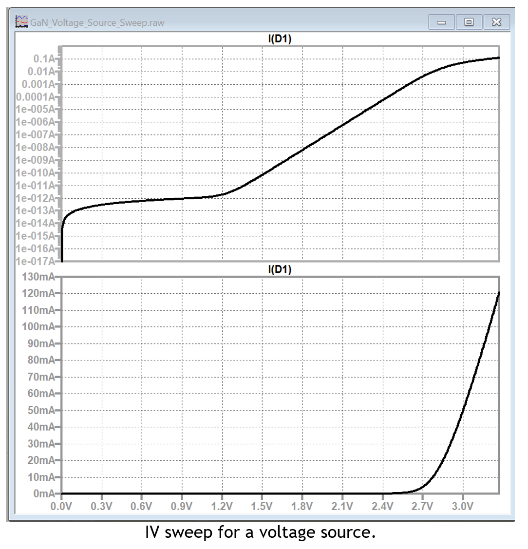
In contrast, the current sweep in the figure below starts at zero and has a 100 μA step size. The current, voltage at the first non-zero datapoint is 100 μA, 2.439297 V and is undefined at lower current.

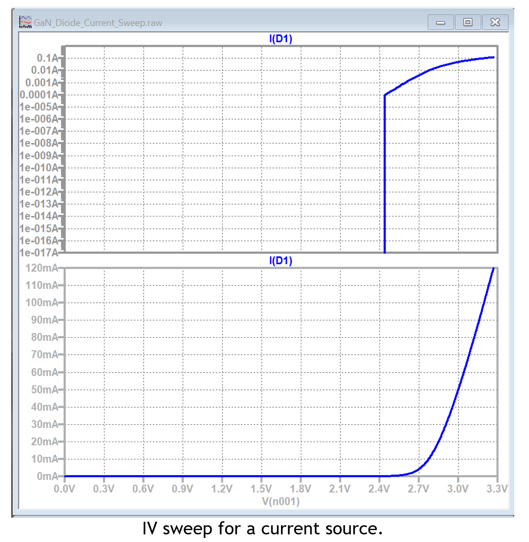
So why do both of these two plots auto range to the same lower limit of 1e-17 A and why does the voltage sweep have that bend at low injection?

The reason is that Spice has a hidden shunt conductance global variable, GMIN, that is used to aid convergence. GMIN is used in many of the device representations in Spice, so although it can be changed this is not advisable.

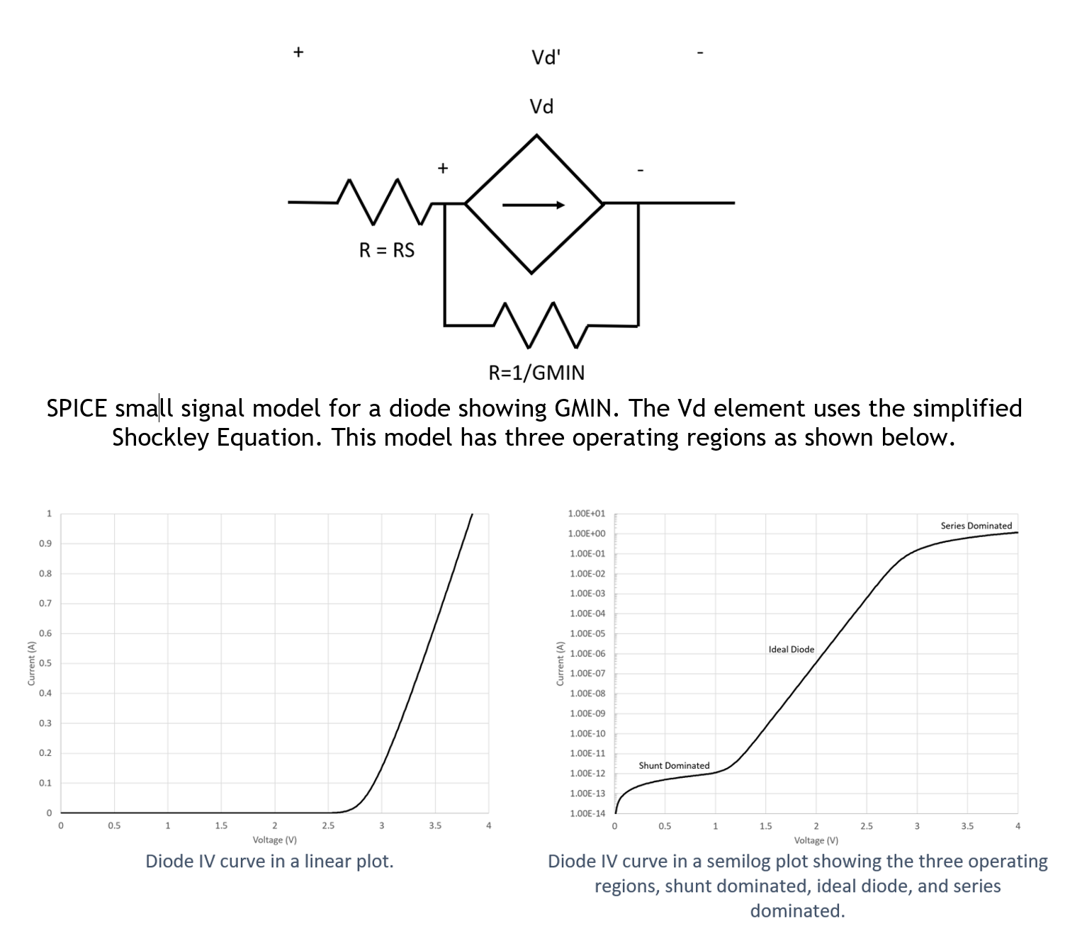
More details on the diode model are discussed in the Luminus Help Center articles “Electrical - What is Current Hogging in Series Parallel Designs?” and “Electrical - How do I insert a diode file into LTspice?”. In this discussion we will show how to modify the current pulse model to get more realistic results.

Be aware that in Spice using 0 as a parameter value is often interpreted as an instruction to use a non-zero default value. This is similar to leaving out a value in a definition string. Spice uses the default value.

Rather than override the value of GMIN, which could have effects on other devices in the model, placing a shunt resistor in parallel with each LED in the schematic is recommended. This will result in a more realistic IV characteristic to match real data as shown in the figure below.

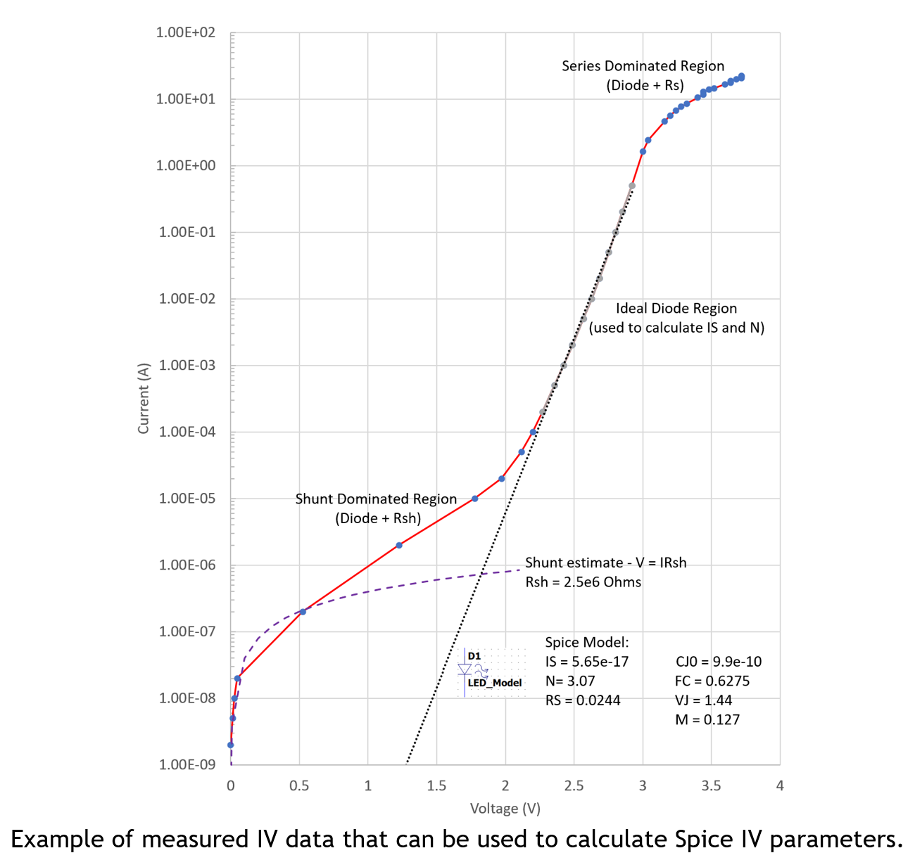
The Spice model without a shunt resistor will give erroneous voltage values below 0.1 mA, the point where the Spice model diverges from the real data.

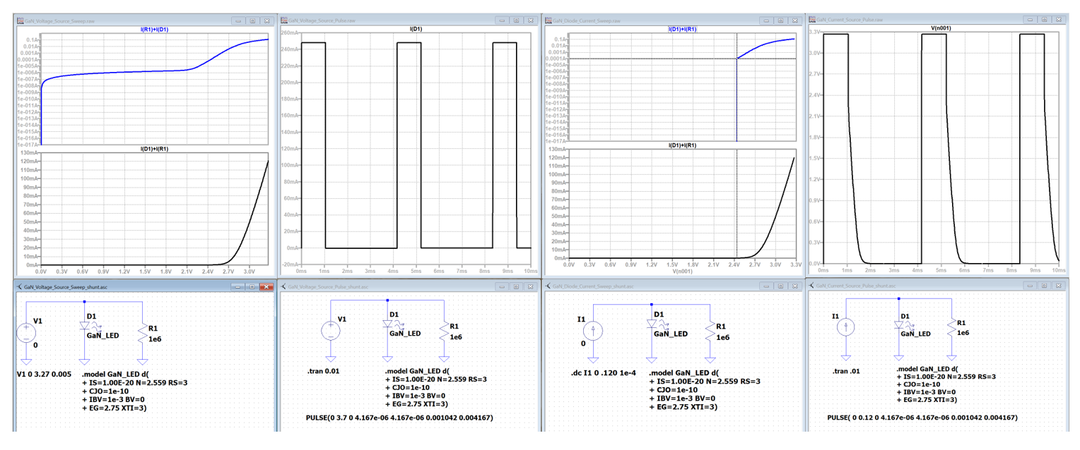
In the figure below we add a 1 MΩ shunt resistance to all four models. We can easily observe changes in the semilog IV plots for the voltage and current sweep and in the current-driven pulse voltage response. The output waveform in the current pulse plot still does not have the right shape. It is pulled down by the shunt resistance but not enough to (correctly) follow the input waveform. This is due to digitization effects in the Spice pulse command.

The figure below is a data dump from the current pulse plot. It shows that the transition to zero current input happens at Isource = 4.2 mA. At 4.2 mA, the voltage is 2.69 V and when the input goes to zero, Spice calculates the RC voltage decay for the equivalent Rs, Rsh, and CJ0 circuit with this voltage as the initial condition.

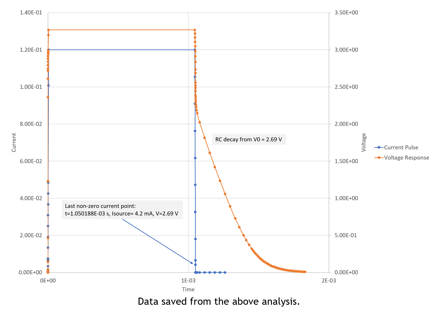
In reality, this type of LED has a fall time on the order of 10 ns and the step size needs to be very small to accurately model the trailing-edge of the pulse response. This is not easily done and would take a ridiculous amount of time, but if done in a way that the last non-zero point in the trailing edge of the pulse were below 1e-8 A, the result would be a square wave.

Spice does not use equal spaced values for input pulse waveforms. It has an adaptive predictor corrector algorithm which is difficult to control. You can specify a maximum step size to increase the sampling rate but there is no guarantee that the algorithm will sample as desired in your region of interest. We tried this with a “suggested” step size maximum of 1e-15 sec and found that the adaptive algorithm generated about 1e-4 A as the last non-zero current in the pulse after running for an hour on a fast computer.

Spice has a feature where you can define a waveform using a PWL file. We tried to generate a pulse with a datapoint specified at 1e-9 A to get a clean waveform. The adaptive algorithm intervened and the lowest current on the pulse trailing edge was 2.8e-6 A rather than the specified 1e-9. There may be other versions of Spice that are more controllable but that is beyond the scope of this article.

[11/23/2022, The PWL method used in "Data Analysis - Using Python to run LTspice as a remote process." appears to give better control over the pulse timing points]

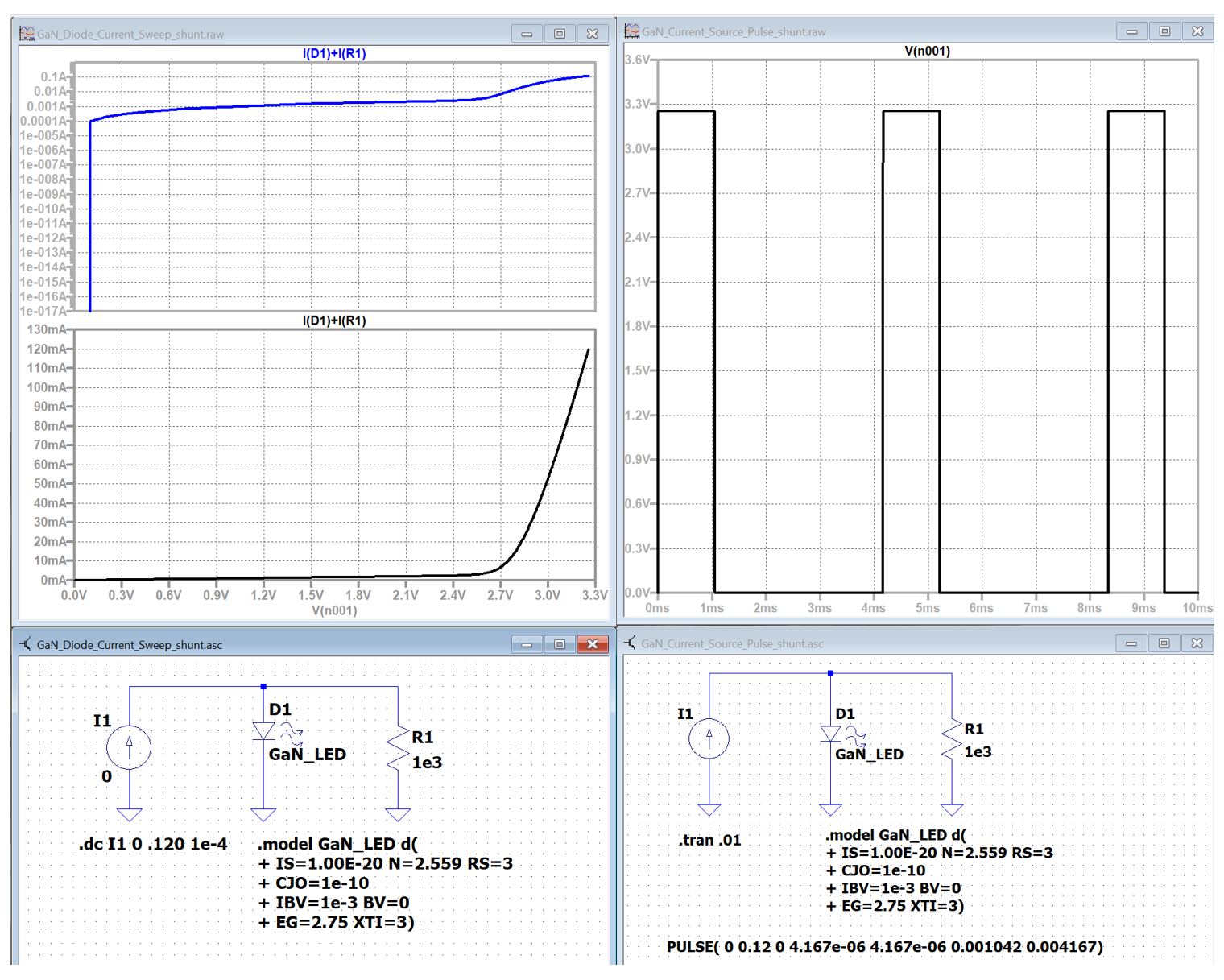
Changing the shunt resistance to a lower value will force the curve to have the (correct) square shape but adds error to the IV curve of the device model.

In the figure below, we have changed the shunt resistance to 1 kΩ and the voltage pulse response is square. However, if you examine the IV curve (bottom left) the current increases from zero volts to the turn-on voltage (about 2.7 V). This is not typical behavior for this type of LED and in fact, this chip would be rejected by the LED die manufacturer and never assembled into an LED package.

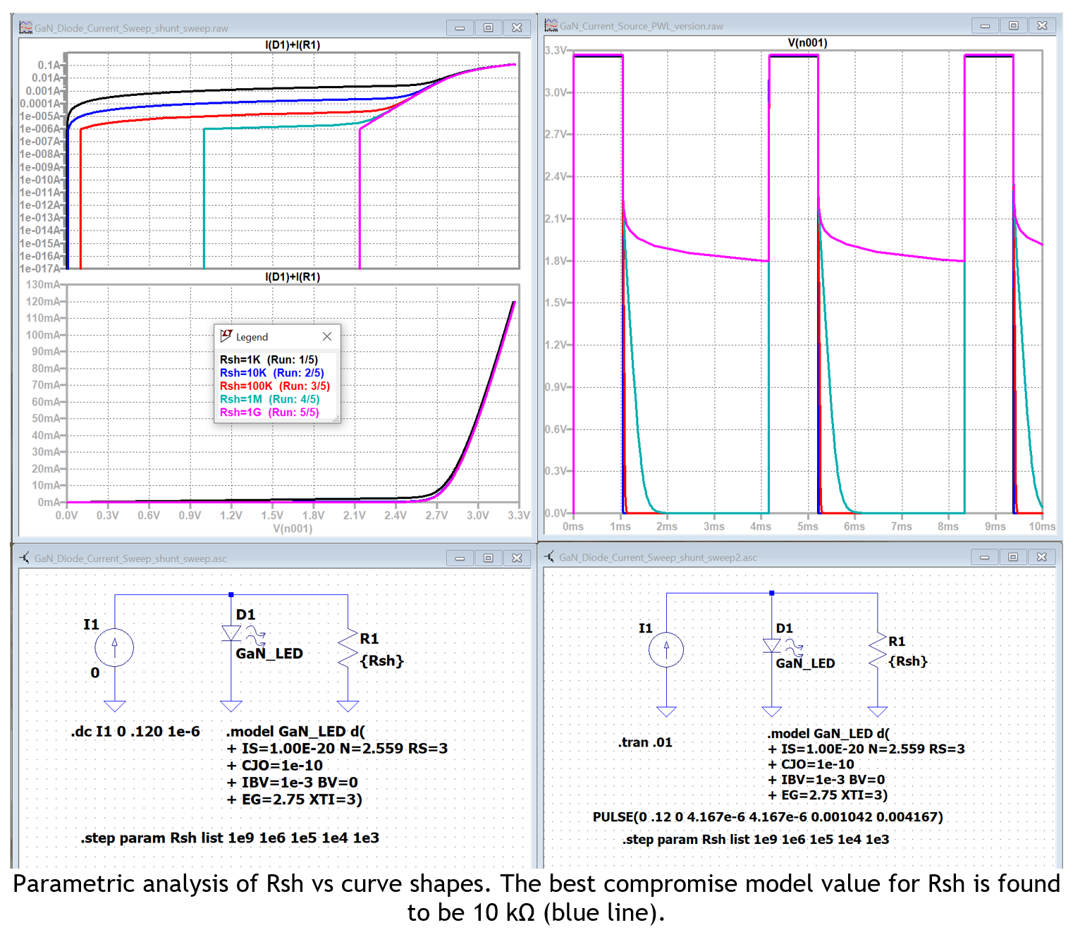
Spice has a number of parametric analysis features, and we use the “.step param list” command in the figure below to visualize the effects of different values of Rsh on squaring up the pulse response. We step through 1e-3, 1e-4, 1e-6, and 1e-9 Ω and find that 1e-4 Ω produces a reasonable waveform shape for both the IV curve and the pulse plot. A 10kΩ shunt value is a little low for real GaN-based LEDs but this model value does not noticeably shift the IV curve and gives a square waveform.

Useful Spice Resources

LTspice Simulator | Analog Devices

LTspice: Adding Third-Party Models | Analog Devices

LTwiki-Wiki for LTspice

LTspice Annotated and Expanded Help* - LTwiki-Wiki for LTspice

Simon Bramble | Analog Circuit Design | LTspice Tutorials

LTspice groups.io Group

Related articles